Overview: Package Purpose
Health departments commonly seek clusters of cases in space and time, as cases occurring within similar time frames in nearby locations could signal outbreaks or other events of public health importance. The input data intended for the current package are typically counts of outcomes for syndromic categories such as emergency department visits for selected infectious diseases, overdoses, or other harms. However, the package may be applied to seek clusters of other types of count data whose observations have space and time descriptors. The following paragraphs briefly summarize the cluster-finding method.
The scan statistic is a widely used method for detecting clusters. For a given outcome, the method works by testing many candidate regions for high observed counts of that outcome and identifying regions with unusually high counts relative to expected levels. In many applications including the current one, expected counts are derived from a baseline set of historical data. The most anomalous regions are then evaluated for statistical significance and potential alerting. This approach is implemented in the SaTScan software (www.satscan.org), which uses a moving cylindrical window over space and time. The base of each cylinder defines a geographic area, while its height represents a time interval. For each cylinder, the observed number of cases is compared with the expected count using a test statistic. The cylinder with the maximum value of the scan statistic defines a candidate cluster.
Because the distribution of the maximum scan statistic is not available in closed form, SaTScan estimates statistical significance using Monte Carlo simulation. That is, it repeatedly generates simulated datasets under a null model and compares the observed cluster to this reference distribution. The approach implemented in this package replaces these repeated simulations with an immediate significance assessment based on spline functions trained on a large set of archived SaTScan results. The user chooses a spline corresponding to a significance level; this spline defines a threshold for each possible observed count. For each candidate cluster, an alert is issued if its observed count exceeds the corresponding threshold. This method reduces computation time while providing a practical approximation to the standard SaTScan significance test, enabling rapid, on-demand cluster detection across outcomes and time scales. The approach is faster than using conventional repeated trials and provides epidemiologists with a proxy method to obtain clusters on demand, for any outcome, and of any duration.
Requirements for this scan statistic implementation are:
assignment of the observed data to geographic regions with centroid point locations for distance calculations to enable expanding cylinder scans
observed counts of the data in each region for each time step
corresponding expected counts of the data, estimated from baseline data
distances between the regions
Package functionality
The current package provides utilities for cluster detection on location-date-count surveillance data. It supports:
- building location distance structures (matrix and sparse list forms),
- computing baseline/test summaries and visualization-ready outputs,
- running a full clustering workflow through
find_clusters(), - using lower-level functions when step-wise control is needed,
- simulating cluster injections for testing workflows.
This vignette demonstrates all exported functions, with emphasis on
the recommended wrapper: find_clusters().
Technical Requirements to Enable Cluster Detection in User Data
find_clusters() expects a data frame with at least these
columns:
-
location: character location identifier, -
date:Date(orIDate) values, -
count: non-negative counts. Dates and locations with zero counts need not be provided. For many outcomes, counts are zero for the majority of locations in most dates and locations. The package code accounts for all date/location pairs.
# use the built in example_count_data
cases <- data.table::as.data.table(example_count_data)

head(cases)
#>    location       date count
#>      <char>     <IDat> <int>
#> 1:    39001 2024-10-01     3
#> 2:    39001 2024-10-02     1
#> 3:    39001 2024-10-03     2
#> 4:    39001 2024-10-04     5
#> 5:    39001 2024-10-05     4
#> 6:    39003 2024-10-01     4
Date helper functions: These are show here for reference, but not usually needed in application:
detect_date <- max(cases$date)

# get the test dates, given a detect date and test_length
get_test_dates(detect_date, test_length = 7)
#> [1] "2025-01-30" "2025-01-31" "2025-02-01" "2025-02-02" "2025-02-03"
#> [6] "2025-02-04" "2025-02-05"

# get the baseline dates, given a detect date, test and baseline length
get_baseline_dates(
  detect_date,
  test_length = 7,
  baseline_length = 90,
  guard = 0
) |> head()
#> [1] "2024-11-01" "2024-11-02" "2024-11-03" "2024-11-04" "2024-11-05"
#> [6] "2024-11-06"
Distance Structures for Geographic Scanning
The scanning process requires distances between locations to enable systematic scanning of expanding cylinders in space. This package provides two ways to provide these distances:
Full Distance Matrix Functions:
The functions tract_distance_matrix(),
zip_distance_matrix(),
county_distance_matrix(), and
state_distance_matrix() provide full pairwise distance
matrices (i.e. size N x N, where N is the
number of locations, and each cell is the distance between the centroids
of any paired locations:
zip_dm <- zip_distance_matrix("DC")
dim(zip_dm$distance_matrix)
#> [1] 246 246

county_dm <- county_distance_matrix("RI", source = "tigris")
dim(county_dm$distance_matrix)
#> [1] 5 5
us_distance_matrix() is a special function available for
generating pairwise distance between all U.S. counties, but is typically
too large for routine examples:
us_dm <- us_distance_matrix()Limited Distance Lists
For applications with many hundreds of locations, the above matrices
may contain many location-pair estimations that are not needed because
the distance between the locations exceeds the cluster radius that is
appropriate. As a result, these matrices can be slower to compute and
many of the cells are unnecessary. Therefore, we provide an alternate
representation via the function create_dist_list() . The
output of this function is a list of vectors containing the
nearby neighbor locations for each data
location, where “nearby” means within a user-provided threshold. The
example below returns a list of all counties within 25 miles for every
county in Rhode Island. This list is adequate for detection of clusters
whose radius is at most 25 miles. For many outcomes, users do not seek
clusters whose geographic extent exceed a threshold.
In summary, the matrix functions return all pairwise distances in a
large, square matrix, while create_dist_list() returns only
a sparse list of within-threshold neighbors (sparse list). The sparse
lists are often faster/lighter for large geographies.
county_list <- create_dist_list(
  level = "county",
  st = "RI",
  threshold = 25
)
length(county_list)
#> [1] 5
head(county_list[[1]])
#>    44009    44005    44003
#>  0.00000 18.89133 19.34145
For more detailed information on creating distance objects, see
vignette("distance_objects")
Main Wrapper: find_clusters()
The primary user-facing function is find_clusters. This
function executes the following component steps:
- build baseline/test count grids,
- aggregate nearby-location counts by distance,
- compute observed and expected values,
- apply spline-derived significance thresholds,
- compress candidate clusters to remove less significant ones and avoid overlap,
- append all location-level counts for retained clusters.
Preparing Inputs
For any distance object (matrix or sparse list), location names must
match the location column in your case data.
Key Parameters in find_clusters()
Required:
| Parameter | Purpose | Comment |
|---|---|---|
cases |
Input location-date-count data | Include only rows whose count is positive. |
distance_matrix |
Named matrix (dense) or named list (sparse) of distances | Used for scanning to include progressively closer locations. |
detect_date |
End date for the detection window | Function will return only clusters ending on this date. |
Optional:
| Parameter | Purpose | Comment |
|---|---|---|
spline_lookup |
Spline threshold table (NULL, built-ins
"05", "01", "005",
"001", or custom frame) |
Derived from SaTScan cluster output runs with p-values of 0.05, 0.01, 0.005, and 0.001, to emulate those sensitivity requirements |
baseline_length |
Number of days in baseline period | Default is 90 days; can use larger intervals if available in
cases. |
max_test_window_days |
Maximum test window size (days) | Number of days that a cluster can include, i.e. max cylinder height. |
guard_band |
Gap between baseline and test windows | Default is 0 days; can be used to separate test window from baseline. |
distance_limit |
Max cluster radius in same units as distances | Mean maximum distance from centroid to cluster members. |
baseline_adjustment |
Expected-value handling ("add_one",
"add_one_global", "add_test",
"none") |
Select “add-test” to agree with SaTScan space-time permutation option “add-one” to add a baseline count when needed |
adj_constant |
Constant used when adjustment requires additive offset | default=1; constant added for “add_one” options to avoid division by zero |
min_clust_cases / max_clust_cases
|
Pre-compression observed-count filters | to put a minimum or maximum on number of cluster cases |
return_interim |
Return intermediate objects for debugging/inspection | Lets user inspect intermediate data tables. |
Running find_clusters()
In the argument list below, cluster dimensions are limited to 15 miles from the cluster center and 7 days total including detection date, with a 90-day baseline interval. The baseline_adjustment option is set to “add_test” to include the 7-day test interval counts in the baseline, as in the SaTScan space-time permutation method. The default adjustment “add_one” excludes the test interval and adds one only when needed to avoid division by zero when calculating expected counts.
clusters <- find_clusters(
  cases = cases,
  distance_matrix = dm,
  detect_date = detect_date,
  spline_lookup = "01",
  baseline_length = 90,
  max_test_window_days = 7,
  distance_limit = 15,
  baseline_adjustment = "add_test",
)
Built-In Spline Tables and Example Data
The package ships with spline lookup tables. For observed cluster counts, tables provide significance thresholds approximating p-values of 0.001, 0.005, 0.01, and 0.05:
spline_001spline_005spline_01spline_05
demonstration data, and tables of county and zip code locations (centroids):
example_count_datacountieszipcodes
These can be used directly in workflows, examples, and tests.
Example Cluster Map
library(gsClusterDetect)
library(ggplot2)
library(tigris)
library(sf)
options(tigris_use_cache = TRUE)
# Use example count data to find clusters
d <- example_count_data
dd <- d[, max(date)]
dm <- create_dist_list("county", st = "OH", threshold = 50, )
cl <- find_clusters(d, dm, dd)
# Join locations/clusters to tigris counties shape file
# First get tigris based shape file
oh <- data.table::setDT(
tigris::counties("OH", cb = TRUE, class = "sf")
)
#> | | | 0% | | | 1% | |= | 1% | |= | 2% | |== | 2% | |== | 3% | |=== | 4% | |=== | 5% | |==== | 5% | |==== | 6% | |===== | 7% | |===== | 8% | |====== | 8% | |====== | 9% | |======= | 9% | |======= | 10% | |======== | 11% | |======== | 12% | |========= | 13% | |========== | 14% | |============= | 18% | |============= | 19% | |============== | 20% | |=============== | 21% | |================ | 23% | |================= | 25% | |========================== | 38% | |================================ | 45% | |================================== | 49% | |=========================================== | 61% | |==================================================== | 74% | |==================================================== | 75% | |===================================================== | 76% | |====================================================== | 77% | |====================================================== | 78% | |======================================================= | 79% | |========================================================= | 81% | |=========================================================== | 85% | |============================================================ | 85% | |============================================================ | 86% | |============================================================== | 88% | |=============================================================== | 90% | |=================================================================== | 96% | |======================================================================| 100%
# left join on the cluster location counts, and convert back to sf object
oh <- sf::st_as_sf(
merge(
oh,
cl$cluster_location_counts,
by.x = "GEOID", by.y = "location",
all.x = TRUE
)
)
# Find the number of significant clusters
n_groups <- nrow(cl$cluster_alert_table)
# Get that number of shades of blue
blue_vals <- setNames(
colorRampPalette(c("lightblue", "darkblue"))(n_groups),
sort(unique(na.omit(oh$target)))
)
# Make a simple map of the shape file,
# filling with the target, and then coloring the fill-values
# with the blue vals
ggplot(oh) +
geom_sf(aes(fill = cluster_center), color = "black", linewidth = 0.2) +
scale_fill_manual(values = blue_vals, na.value = NA) +
theme_void() +
theme(legend.position = "none")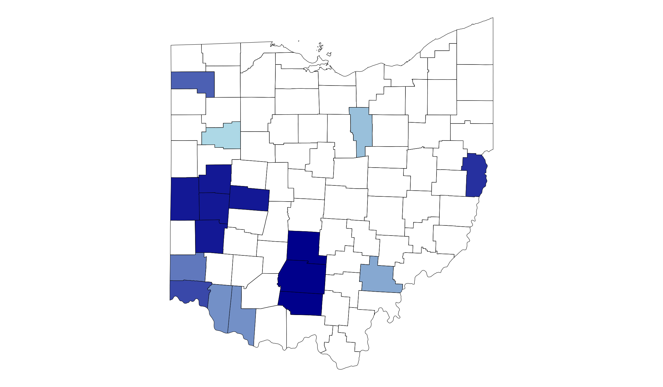
Summary and Plotting Utilities
Create statistical summary of input data:
summary_tbl <- generate_summary_table(
  data = cases,
  end_date = detect_date,
  baseline_length = 90,
  test_length = 7
)
summary_tbl
#>          Statistic (rounded means) Baseline Interval Test Interval
#>                             <char>             <num>         <num>
#>  1:                      Nr. Dates              90.0           7.0
#>  2:                Nr. Total Cases           63803.0        9673.0
#>  3:                  Cases per Day             708.9        1381.9
#>  4:        Nr. Locations with Data              88.0          88.0
#>  5:      Nr. Locations, no records               0.0           0.0
#>  6: Nr. Locs, daily mean 1 or less              15.0           8.0
#>  7:         Nr. Locs, daily mean 2              13.0           6.0
#>  8:       Nr. Locs, daily mean 3-5              29.0          16.0
#>  9:      Nr. Locs, daily mean 6-10              13.0          25.0
#> 10:       Nr. Locs, daily mean >10              18.0          32.0
Create visual heatmap summary of input data to assess suitability for cluster detection. This plot illustrates spread of data counts over locations:
heatmap_data <- generate_heatmap_data(
  data = cases,
  end_date = detect_date,
  baseline_length = 90,
  test_length = 7
)

p_heat <- generate_heatmap(heatmap_data, plot_type = "plotly")
class(p_heat)
#> [1] "plotly"     "htmlwidget"
p_heat
Create time series of aggregated data counts over all locations:
ts_data <- generate_time_series_data(
  data = cases,
  end_date = detect_date,
  baseline_length = 90,
  test_length = 7
)

p_ts <- generate_time_series_plot(ts_data, plot_type = "plotly")
class(p_ts)
#> [1] "plotly"     "htmlwidget"
p_ts